4.3. Project: Bond Graph

This project was created as part of the Computational Physiology module in the MedTech CoRE Doctoral Training Programme.

This project requires you to put together what you have learned in the tutorials to define a complete workflow which will create the Hill muscle model using the Bond Graph technique to simulate the human gait motion.

4.3.1. Outline

The Hill muscle model showed in Fig. 4.12 can be represented with the Bond Graph technique using 1-junction for common velocity point, 0-junction for common force point, a tension source SE for the contractile tension, a resistor R for the mechanical damper, two capacitors C for springs, and a mass I representing the muscle mass.

In this project we create the Hill muscle model using the Bond Graph technique.

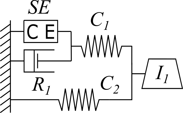
Fig. 4.12 The Hill model with five basic elements: contractile element, CE; damping element, \(R_{1}\); series elastic element, \(C_{1}\); parallel elastic element, \(C_{2}\); and inertial element, \(I_{1}\).

4.3.2. Tips for completing the project

• Junctions: 1-junction and 0-junction are the fundamental elements for building Bond Graph models from schematics. By identifying the junctions in the schematic we can come up with the network topology, which helps us to plug in the rest of the elements to the model.
• Contractile element: The contractile element CE is the active element in an extrafusal motor unit. It corresponds to the role played by voltage in an electronic circuit. CE responds to motoneuron inputs by contracting. Thus, the tension SE that it produces always acts to try to shorten the muscle. CE is incapable to produce an extension force. Here, we assume the force is constant with given value of \(1\) J.m^-1.
• Elastic elements: A muscle when passively stretched exhibits an elastic restoring force that tends to return the muscle to its original length. In part this force is due to stretching the connective tissue that surrounds the muscle fibers. In part it may be due to stretching the tendons which terminate muscle tissue and attach it to the bone. There is a reason to believe that the muscle fibers themselves are at least partly elastic. It is this elastic restoring force that is represented by the elastic elements (springs) in the Hill model. It is not completely correct to assign these elements to any particular physical source, but we may regard the \(C_{1}\) as being mostly due to the connective tissues and the \(C_{2}\) as being primarily dominated by tendon fibers terminating specific motor units. We should note that \(C_{1}\) and \(C_{2}\) are functions of lengths and therefore are non-linear springs. However, in this project we assume they are constants with given value of \(20\) J.m^-2.
• Damping element: It is an empirical factor that muscle tension during contraction and the speed of the contraction are coupled to each other. Hill found that the relation between them follows a characteristic hyperbolic equation, now known as Hill’s equation. Similar to elastic elements, the damper coefficient \(R_{1}\) is a function of the contraction speed, therefore is a nonlinear damper. However, in here we assume it is constant with given value of \(10\) J.s.m^-2.
• Inertial element: This element is representing the muscle mass. Here, we assume it is \(1\) J.s² .m^-2.

The full Bond Graph muscle model is shown in Fig. 4.13.

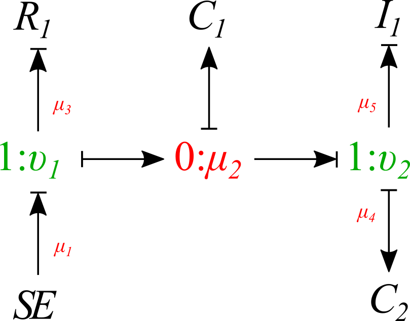
Fig. 4.13 Full Bond Graph muscle model.

4.3.3. Simulation

Using the Bond Graph model, now we can derive the equations and implement them in OpenCOR. The equations that we are looking for are: conservation of flow for 0-junctions, conservation of energy for 1-junctions, and constitutive relations for the springs, the damper and the mass. The input boundary condition for solving this system of ODEs is the contractile element or SE in the Bond Graph model. By running the simulation, you would be able to plot the force, velocity and displacement for the muscle in time.